Most explanations of softmax regression start too late. They present the formula, maybe mention normalization, and move on. That is efficient, but it hides the idea.

The cleaner way to think about it is to start one step earlier. First understand logistic regression properly. And to understand logistic regression properly, start from odds.

So the real chain is:

$$ \text{probability} \to \text{odds} \to \text{log-odds} \to \text{logistic regression} \to \text{softmax regression}. $$

Once that chain is visible, softmax stops looking like a mysterious trick. It becomes the obvious multiclass continuation of the same probabilistic story.

If you want the full runnable walkthrough, the companion notebook lives on Kaggle:

https://www.kaggle.com/code/lyhatt/softmax-from-logistic-regression

That notebook was assisted by AI tools. This note is the more streamlined written version.

Start with Probability, Then Ask for More Structure

Suppose we have a binary outcome. Let

$$ p = P(y=1 \mid x) $$

be the probability that the positive class occurs given the input $x$.

Probability is easy to interpret, but it is not yet the best thing to model. A slightly more structured object is the odds:

$$ \text{odds} = \frac{p}{1-p}. $$

The odds tell us how much more likely the positive event is than the negative one.

Some quick examples help. If $p = 0.5$, then the odds are $1$. If $p = 0.8$, then the odds are $\frac{0.8}{0.2} = 4$. If $p = 0.2$, then the odds are $\frac{0.2}{0.8} = 0.25$. So odds greater than $1$ favor the positive class, odds less than $1$ favor the negative class, and odds equal to $1$ mean the two classes are balanced.

This is already useful, but there is a problem. Odds are always positive, so they live on $(0,\infty)$. A plain linear model

$$ w^T x + b $$

lives on the whole real line, from $-\infty$ to $\infty$. Those two spaces do not match well. If we want a linear model, odds are the wrong coordinates.

The Core Move: Take Logarithms

To fix this, we take the logarithm of the odds:

$$ \log \frac{p}{1-p}. $$

This quantity is the log-odds, also called the logit.

Why is this useful? Because odds are constrained to be positive, but log-odds can be any real number. A logit of $0$ corresponds to $p=0.5$, positive logits correspond to probabilities above $0.5$, and negative logits correspond to probabilities below $0.5$. This is the key move. The logarithm converts a positive ratio into a quantity that can now range over the whole real line. That means a linear model suddenly fits naturally:

$$ \log \frac{p}{1-p} = w^T x + b. $$

This is logistic regression in its cleanest form. The model says: not that the probability is linear, but that the log-odds are linear.

Now Solve for the Probability

Now let us solve for $p$ carefully. Start with

$$ \log \frac{p}{1-p} = w^T x + b. $$

Exponentiate both sides:

$$ \frac{p}{1-p} = e^{w^T x + b}. $$

This is where the exponential enters the story, and it is doing real mathematical work. It appears because it is the inverse of the logarithm, because it guarantees the odds stay positive, and because it converts an unrestricted real-valued score into a valid positive ratio.

Now multiply both sides by $(1-p)$:

$$ p = (1-p)e^{w^T x + b}. $$

Expand the right-hand side:

$$ p = e^{w^T x + b} - pe^{w^T x + b}. $$

Collect the $p$ terms:

$$ p + pe^{w^T x + b} = e^{w^T x + b}. $$

Factor out $p$:

$$ p\left(1 + e^{w^T x + b}\right) = e^{w^T x + b}. $$

So

$$ p = \frac{e^{w^T x + b}}{1 + e^{w^T x + b}}. $$

Divide numerator and denominator by $e^{w^T x + b}$:

$$ p = \frac{1}{1 + e^{-(w^T x + b)}}. $$

This is the sigmoid form of logistic regression:

$$ p = \sigma(w^T x + b). $$

This is the full derivation. The sigmoid is not a decorative choice. It is what falls out when a linear model is placed on the log-odds.

What the Sigmoid Is Really Doing

The sigmoid takes a real-valued score and maps it to a number between $0$ and $1$:

$$ \sigma(z) = \frac{1}{1+e^{-z}}. $$

Here $z = w^T x + b$ is often called the logit.

The interpretation is immediate once you remember that $z$ is a logit. If $z \gg 0$, then $\sigma(z)$ is close to $1$. If $z = 0$, then $\sigma(z)=0.5$. If $z \ll 0$, then $\sigma(z)$ is close to $0$. So the sigmoid is the map from linear evidence to probability. That is why logistic regression has the familiar S-curve.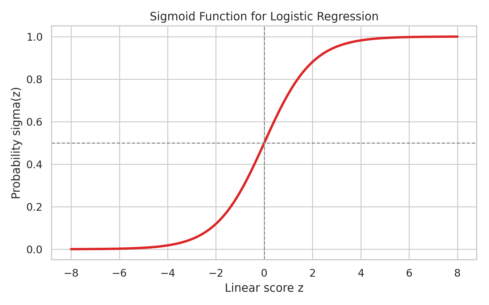

The Model Needs a Learning Signal

Once the model outputs probabilities, the next question is: what objective should it optimize? Logistic regression uses the Bernoulli likelihood. For one example with label $y \in {0,1}$ and predicted probability $\hat{y}$,

$$ P(y \mid x) = \hat{y}^y(1-\hat{y})^{1-y}. $$

Taking logs gives the log-likelihood:

$$ \log P(y \mid x) = y \log \hat{y} + (1-y)\log(1-\hat{y}). $$

For $m$ observations, the negative average log-likelihood becomes the binary cross-entropy:

$$ L = -\frac{1}{m} \sum_{i=1}^m \left[y^{(i)} \log \hat{y}^{(i)} + (1-y^{(i)})\log(1-\hat{y}^{(i)})\right]. $$

This loss is worth staring at for a moment. It tells you exactly what the model fears: confident mistakes.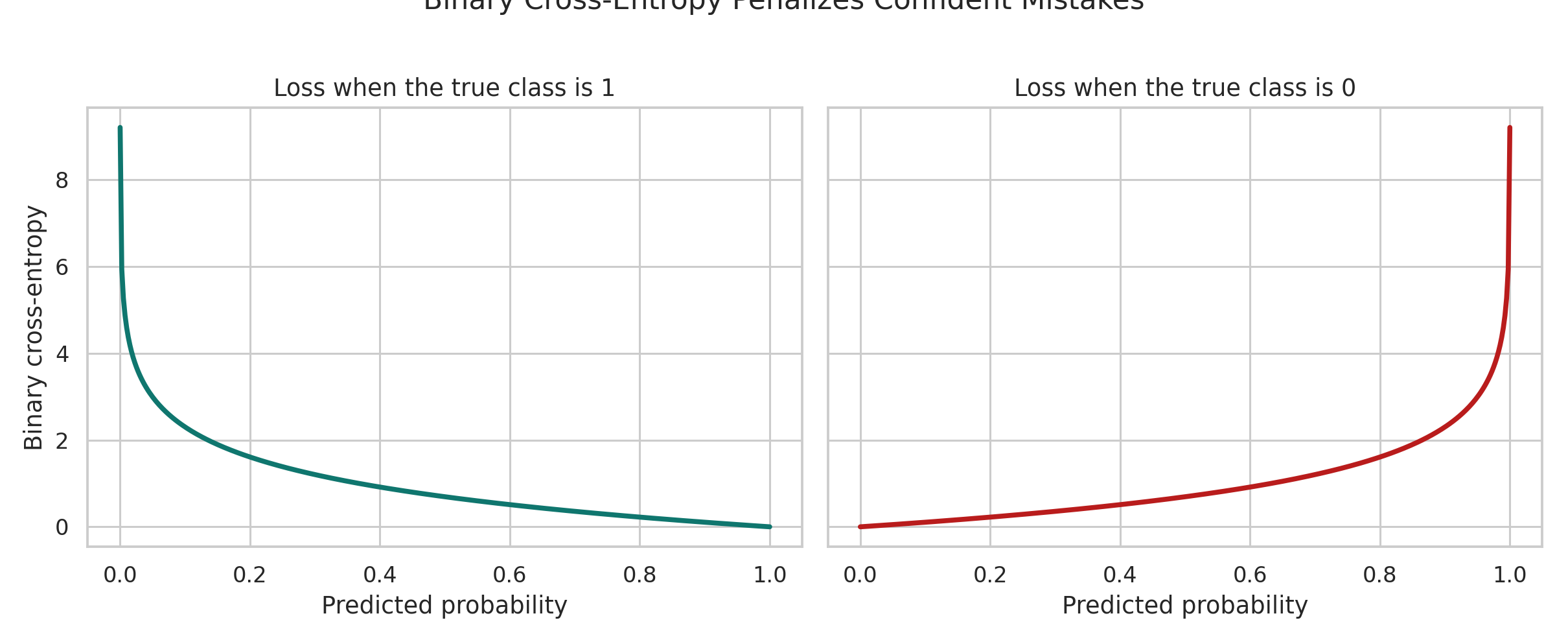

That is the right behavior for a probabilistic model. If it is unsure, the penalty is moderate. If it is confidently wrong, the penalty should explode.

The Optimization Is Still Just Gradient Descent

Once we define the loss, the training rule is still gradient descent. The gradients are

$$ \nabla_w L = \frac{1}{m}X^T(\hat{y}-y), \qquad \nabla_b L = \frac{1}{m}\sum_{i=1}^{m}(\hat{y}^{(i)} - y^{(i)}). $$

So the update step is

$$ w \leftarrow w - \alpha \nabla_w L, \qquad b \leftarrow b - \alpha \nabla_b L. $$

This is worth emphasizing. Logistic regression sounds like a special model class, but algorithmically it is still simple: define probabilities, define a loss, differentiate, and descend.

A Real Binary Example

To make the binary story concrete, we use the Breast Cancer Wisconsin dataset. It has 569 samples, 30 numerical features, and two target classes: 0 for malignant and 1 for benign.

Before fitting anything, it helps to get a feel for the data itself.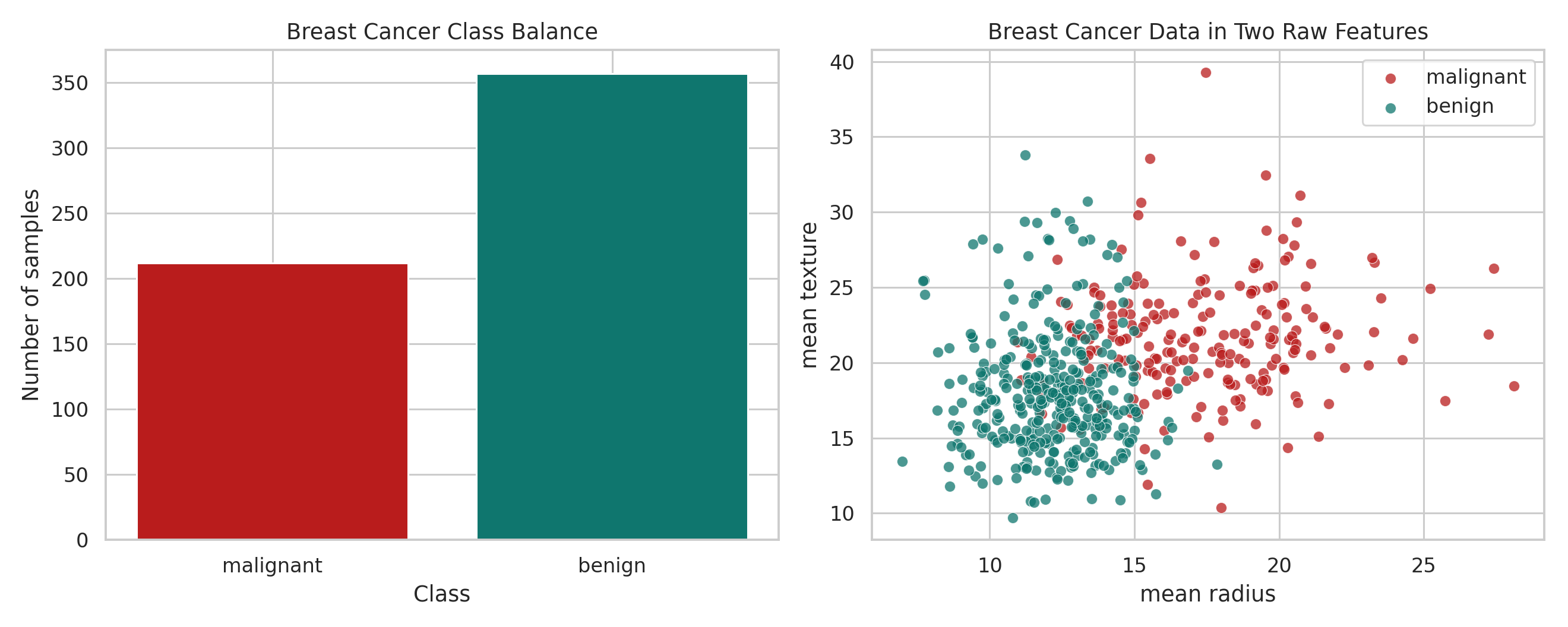

This is just the intuition view. The real training run uses all standardized features, not only the two shown here.

Below is a compact from-scratch implementation of logistic regression with gradient descent:

import numpy as np

def sigmoid(z):
    return 1.0 / (1.0 + np.exp(-z))

def binary_cross_entropy(y_true, y_prob):
    eps = 1e-12
    y_prob = np.clip(y_prob, eps, 1 - eps)
    return -np.mean(y_true * np.log(y_prob) + (1 - y_true) * np.log(1 - y_prob))

def train_binary_logistic(X, y, learning_rate=0.1, epochs=1500):
    n_samples, n_features = X.shape
    weights = np.zeros(n_features)
    bias = 0.0
    history = []

    for _ in range(epochs):
        logits = X @ weights + bias
        probs = sigmoid(logits)
        error = probs - y
        grad_w = X.T @ error / n_samples
        grad_b = np.mean(error)
        weights -= learning_rate * grad_w
        bias -= learning_rate * grad_b
        history.append(binary_cross_entropy(y, probs))

    return weights, bias, np.array(history)

The training loss falls in the way we expect: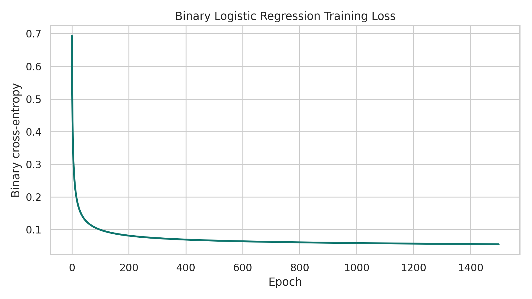

If we restrict ourselves to two features, we can also draw the probability surface directly: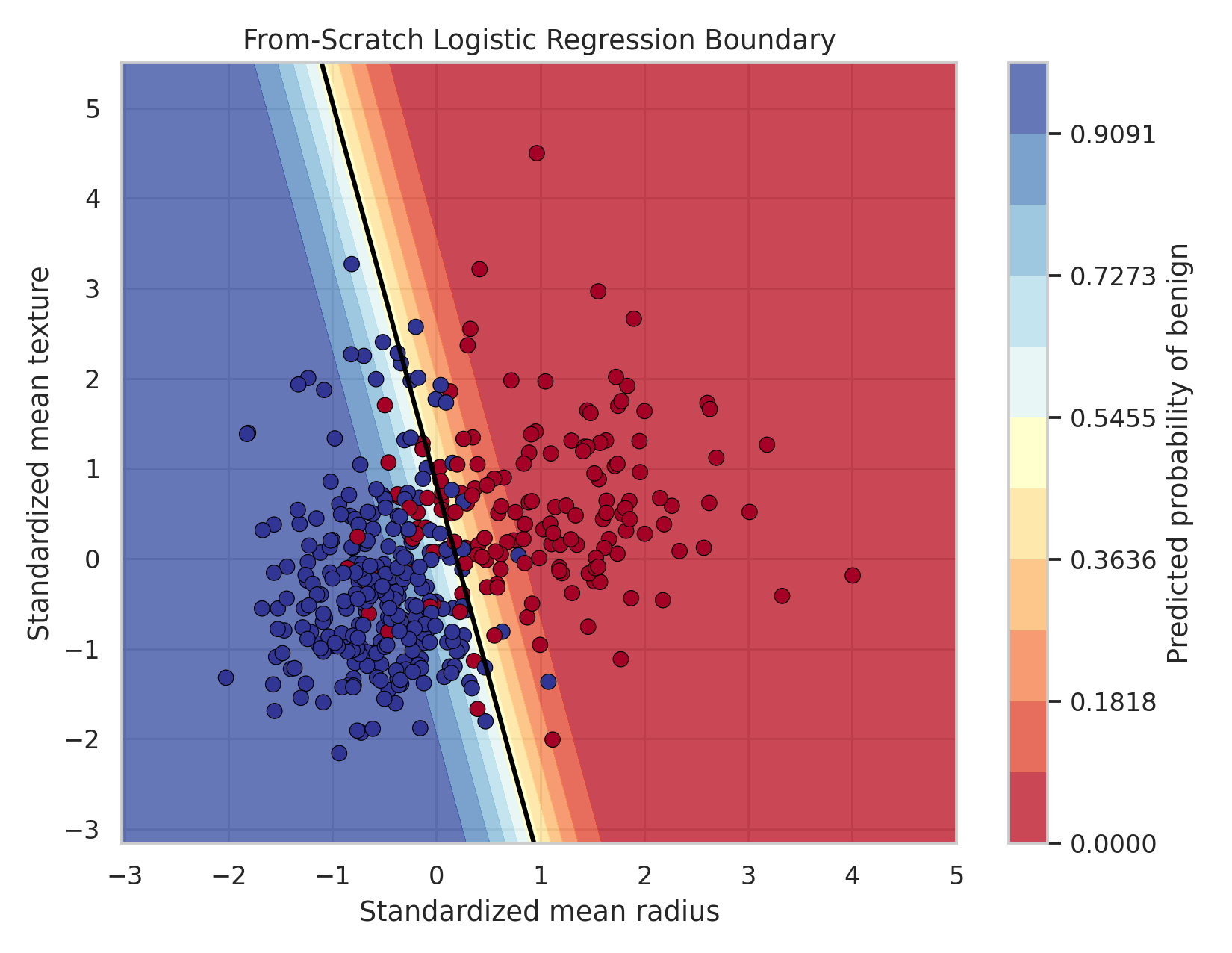

That is enough for the binary story. The point is not to pile up diagnostics. The point is to see that logistic regression turns a linear score into a probability, and then learns that mapping through gradient descent.

The Jump to Many Classes

Now comes the real question: what changes when there are not two classes, but many?

In binary logistic regression, we can think of the model as comparing two outcomes. The odds are

$$ \frac{p}{1-p}. $$

That ratio is already a comparison between classes. Softmax keeps the same spirit, but scales it from two classes to $K$ classes.

One useful way to think about this is to stop thinking in terms of labels first and think in terms of score comparisons.

Imagine an image classifier. A certain image might look a bit like a car, somewhat like a truck, and definitely not like a frog. In that situation, the model does not begin with probabilities. It begins with raw scores. Maybe the car score is high, the truck score is also fairly high, and the frog score is very low. That is already a meaningful picture. "Car versus truck" is a hard distinction because those classes can share visual structure. "Car versus frog" is easier because the scores should separate much more aggressively.

Softmax takes exactly this kind of score vector and says: fine, now turn those relative preferences into a probability distribution.

Suppose each class $k$ gets its own score

$$ z_k. $$

If we want a multiclass probability model, the outputs should satisfy three requirements. Each probability must be positive, all probabilities must sum to $1$, and a larger score should correspond to a larger probability. The exponential is the natural choice here because $e^{z_k}$ is always positive, because if $z_a > z_b$ then $e^{z_a} > e^{z_b}$, and because exponentials turn unrestricted scores into positive quantities that can be normalized.

So we first define unnormalized class weights:

$$ \tilde{p}_k = e^{z_k}. $$

These are not probabilities yet, because they do not sum to $1$. So we normalize them:

$$ p_k = \frac{e^{z_k}}{\sum_{j=1}^{K} e^{z_j}}. $$

That normalization step is softmax.

Why Exponentials Keep Showing Up

At this point the exponential should no longer feel mysterious.

For logistic regression, we start from log-odds, exponentiation recovers the odds, and the final algebra gives the sigmoid probability. For softmax regression, we start from a score for each class, exponentiation turns each score into a positive class weight, and normalization turns those positive weights into a probability distribution. It is the same structural tool in both models: take unrestricted scores, convert them into positive quantities, and only then interpret them probabilistically.

There is also an intuitive reason practitioners like this view. A difference in score should matter more when it is decisive and less when two classes are nearly tied. Exponentials amplify those differences in a smooth way. If "car" scores only slightly above "truck", the probabilities stay competitive. If "car" scores far above "frog", the probability mass shifts much more aggressively.

Softmax Actually Contains Logistic Regression

Softmax is the multiclass extension of logistic regression, and we can show that mathematically.

Take the two-class case with scores $z_0$ and $z_1$. Then softmax gives

$$ p_1 = \frac{e^{z_1}}{e^{z_0} + e^{z_1}}. $$

Factor out $e^{z_1}$ in the denominator:

$$ p_1 = \frac{e^{z_1}}{e^{z_1}\left(e^{z_0-z_1}+1\right)} = \frac{1}{1 + e^{z_0-z_1}}. $$

Equivalently,

$$ p_1 = \frac{1}{1 + e^{-(z_1-z_0)}}. $$

This is exactly a sigmoid in the score difference $z_1-z_0$.

That is the bridge. Logistic regression is the binary special case, and softmax regression is the multiclass generalization.

The Multiclass Loss Is the Same Idea Again

In the multiclass setting, the true label is represented as a one-hot vector. If $Y$ is the one-hot target matrix and $P$ is the predicted softmax probability matrix, then the multiclass cross-entropy is

$$ L = -\frac{1}{m}\sum_{i=1}^{m}\sum_{k=1}^{K} y_k^{(i)} \log p_k^{(i)}. $$

This is the same negative log-likelihood idea again, just written for many classes instead of two.

The gradient keeps a remarkably clean form:

$$ \nabla_W L = \frac{1}{m}X^T(P-Y), \qquad \nabla_b L = \frac{1}{m}\sum_{i=1}^{m}(P^{(i)} - Y^{(i)}). $$

So the optimization rule is still gradient descent:

$$ W \leftarrow W - \alpha \nabla_W L, \qquad b \leftarrow b - \alpha \nabla_b L. $$

So the whole picture survives the transition almost unchanged. The binary weight vector becomes a class-wise weight matrix, and everything else follows.

A Real Multiclass Example

For the multiclass example, we use the Digits dataset. This is much more appropriate for softmax because it contains ten classes instead of two.

Each digit image is an $8 \times 8$ grayscale grid, flattened into a 64-dimensional vector.

Before fitting the model, it is worth seeing both raw samples and class averages: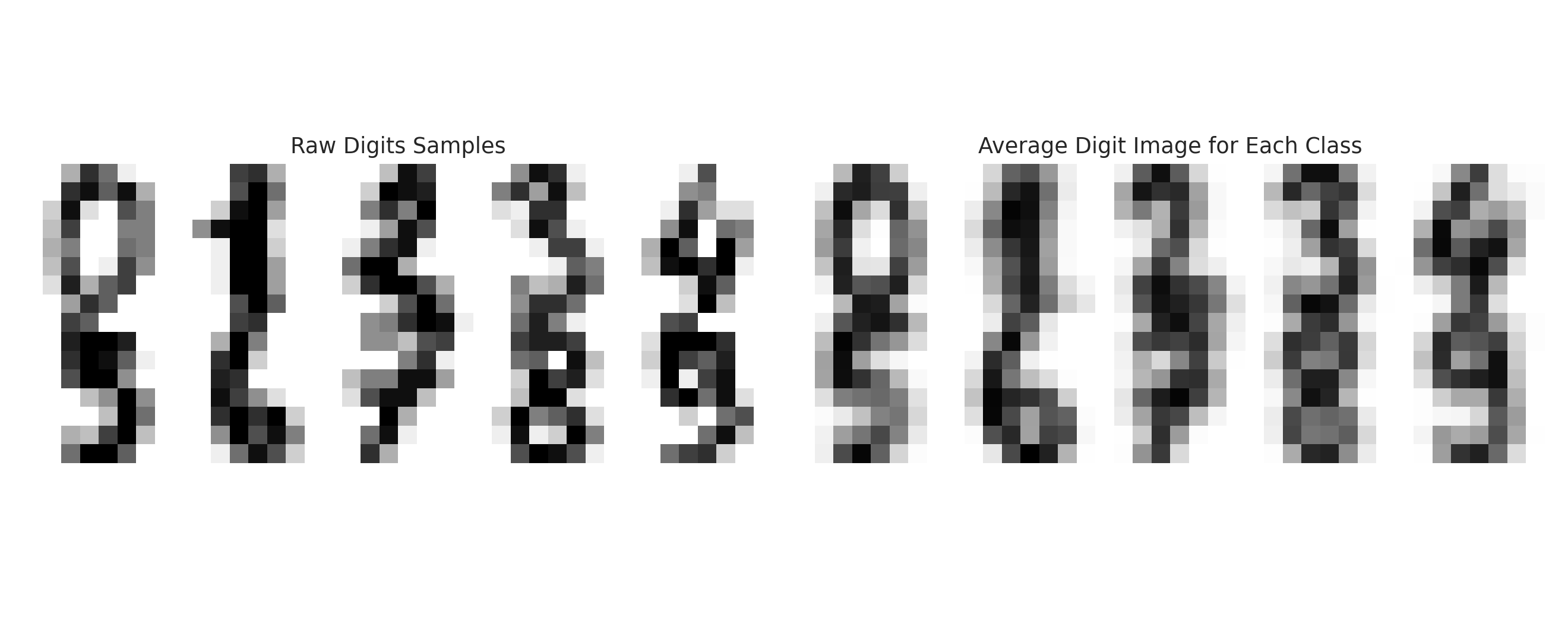

Here is a compact from-scratch softmax regression implementation:

import numpy as np

def softmax(logits):
    shifted = logits - np.max(logits, axis=1, keepdims=True)
    exp_logits = np.exp(shifted)
    return exp_logits / np.sum(exp_logits, axis=1, keepdims=True)

def multiclass_cross_entropy(y_one_hot, probs):
    eps = 1e-12
    probs = np.clip(probs, eps, 1 - eps)
    return -np.mean(np.sum(y_one_hot * np.log(probs), axis=1))

def train_softmax_regression(X, y, learning_rate=0.1, epochs=3000):
    n_samples, n_features = X.shape
    n_classes = len(np.unique(y))
    weights = np.zeros((n_features, n_classes))
    bias = np.zeros(n_classes)
    y_one_hot = np.eye(n_classes)[y]
    history = []

    for _ in range(epochs):
        logits = X @ weights + bias
        probs = softmax(logits)
        error = probs - y_one_hot
        grad_w = X.T @ error / n_samples
        grad_b = np.mean(error, axis=0)
        weights -= learning_rate * grad_w
        bias -= learning_rate * grad_b
        history.append(multiclass_cross_entropy(y_one_hot, probs))

    return weights, bias, np.array(history)

How to Visualize Softmax Honestly

Sigmoid has a universal curve. Softmax does not.

So the honest softmax visualization is not a fake one-dimensional curve. It is a sample-level transformation: start from a real digit image, compute one raw logit per class, and then exponentiate and normalize into probabilities. That is exactly what the next figure shows: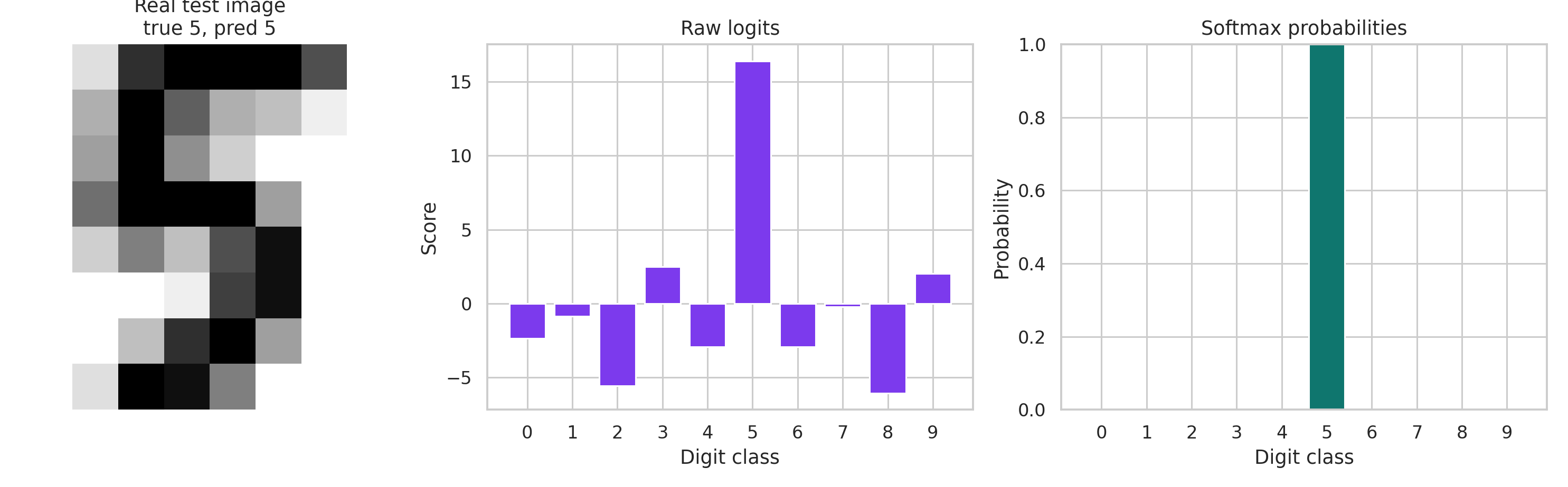

That is the mental model to keep: softmax takes a vector of scores and turns it into a probability distribution.

In other words, softmax is less about drawing one magical curve and more about resolving competitions among classes. Some competitions are close, like car versus truck. Some are not, like car versus frog. The probability vector tells us how that competition ended for one specific input.

The training loss on Digits decreases as expected: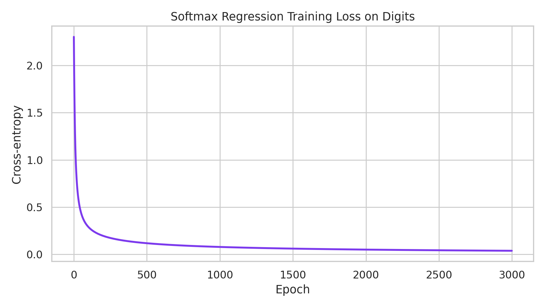

That is enough for the multiclass side as well. Once the reader sees logits become probabilities on a real sample, the central idea has already landed. The remaining plots are useful in a notebook, but they are not necessary in the main essay.

A Few Practical Tradeoffs

This is also a good place to be honest about what logistic regression and softmax regression can and cannot do. They are simple, fast, interpretable, and they produce probabilities directly, which is often exactly what we want. They also work surprisingly well when the classes are close to linearly separable in feature space. But the tradeoff is clear: if the real boundary is highly nonlinear, these models will struggle, the quality of the features matters a great deal, and multiclass confusion often comes from genuinely similar classes rather than from a bug in the formula.

This is also where people usually start reaching for nonlinear models. In deep learning, nonlinear functions become popular precisely because they can build more complex decision boundaries than a single linear logit layer can express. They are often used as activation functions inside deeper networks, and that added nonlinearity is what lets the model represent more complicated structure. But that is really another topic. Here the point is to understand the clean linear baseline first.

That is why these models are such good teaching models and such good baselines. When they succeed, they do so for understandable reasons. When they fail, they usually fail in ways that teach us something about the data.

The Big Picture

At this point the whole thing should feel like one continuous argument, not three unrelated formulas.

We started with probability, then moved to odds:

$$ \frac{p}{1-p}. $$

We took logarithms to obtain log-odds:

$$ \log \frac{p}{1-p}. $$

We modeled the log-odds linearly and solved for the probability, which produced the sigmoid and logistic regression.

Then we asked what happens when there are many classes instead of two. The same need appears again: we must turn unrestricted scores into valid positive ratios, and then normalize them into probabilities. That requirement leads directly to the softmax formula.

So in the end, logistic regression is a model for binary log-odds, softmax regression is the multiclass extension of that same idea, the exponential appears because it converts linear scores into positive ratios, and gradient descent remains the optimization engine underneath both models. That is why logistic regression and softmax regression are best learned together. Once the odds view is clear, softmax stops looking like a memorized formula and starts looking like the inevitable next step.

I think this topic reads better in a slightly stripped-down form. The mathematics should carry most of the weight, and the figures should only appear when they sharpen the argument rather than interrupt it.

If you think there is a better example, a better visualization, or a cleaner way to extend this note, feel free to suggest it. This topic has a nice property: once the odds viewpoint is in place, there are many directions to grow from here.