Most explanations of the Fokker-Planck equation start too late. They write down a partial differential equation for a density, call one term "drift" and the other "diffusion", and move on. That is correct, but it hides where the equation comes from.

The cleaner way to think about it is to start one step earlier, with a single stochastic trajectory. A stochastic differential equation describes one random path. But one path tells you almost nothing. What we usually want is the distribution: given where the system started, where is it likely to be at time $t$? The Fokker-Planck equation is the deterministic law that this distribution obeys.

So the real chain is:

$$ \text{SDE} \to \text{ensemble of paths} \to \text{density } p(x,t) \to \text{Fokker-Planck PDE} \to \text{stationary law}. $$

Once that chain is visible, the equation stops looking like a definition to memorize. It becomes the obvious bookkeeping for how probability mass flows: drift transports it, diffusion spreads it.

This note walks the full path. We start from a concrete SDE and simulate it, watch a cloud of paths turn into a density, derive the Fokker-Planck equation from Ito's lemma, and then solve it from scratch in Python. We finish with an Ornstein-Uhlenbeck example whose answer we know in closed form, so we can check three independent routes against each other.

Run it yourself. Every code block below is collected in a runnable Jupyter notebook: download fokker-planck-sde.ipynb. It only needs numpy and matplotlib (pip install numpy matplotlib), and runs top to bottom.

Start with a Single Trajectory

A stochastic differential equation in one dimension has the form

$$ dX_t = \mu(X_t, t), dt + \sigma(X_t, t), dW_t, $$

where $W_t$ is a Brownian motion. Read it as a rule for taking a small step: over an interval $dt$, the state moves by a deterministic amount $\mu, dt$ (the drift) plus a random kick $\sigma, dW_t$ (the diffusion), where $dW_t$ is a Gaussian increment with mean zero and variance $dt$.

The running example for this note is the Ornstein-Uhlenbeck (OU) process:

$$ dX_t = -\theta X_t, dt + \sigma, dW_t. $$

The drift $-\theta X_t$ pulls the state back toward zero, more strongly the further out it is. The diffusion $\sigma, dW_t$ keeps kicking it away. This tug-of-war between mean reversion and noise is exactly the structure that shows up in interest-rate models, in the velocity of a particle under friction, and in many stationary time series. We will use $\theta = 1$, $\sigma = 1$, and start every path at $X_0 = 2$.

The simplest way to simulate an SDE is the Euler-Maruyama scheme. Discretize time into steps of size $\Delta t$ and replace the differentials by increments:

$$ X_{k+1} = X_k + \mu(X_k, t_k), \Delta t + \sigma(X_k, t_k), \sqrt{\Delta t}; Z_k, \qquad Z_k \sim \mathcal{N}(0, 1). $$

The only subtlety is that the random increment scales as $\sqrt{\Delta t}$, not $\Delta t$. That is the signature of Brownian motion: over a window of length $\Delta t$ the displacement has standard deviation $\sqrt{\Delta t}$, so variance grows linearly in time.

import numpy as np

def euler_maruyama(mu, sigma, x0, T, dt, n_paths, rng):
    n_steps = int(T / dt)
    X = np.full(n_paths, float(x0))
    traj = np.empty((n_steps + 1, n_paths))
    traj[0] = X
    for k in range(n_steps):
        t = k * dt
        Z = rng.standard_normal(n_paths)
        X = X + mu(X, t) * dt + sigma(X, t) * np.sqrt(dt) * Z
        traj[k + 1] = X
    return traj

theta, sigma_ou, x0 = 1.0, 1.0, 2.0
mu = lambda x, t: -theta * x
sig = lambda x, t: sigma_ou

rng = np.random.default_rng(0)
traj = euler_maruyama(mu, sig, x0, T=4.0, dt=1e-3, n_paths=20000, rng=rng)

A handful of these paths, plotted over time, all start at $2$ and get dragged toward zero while jittering: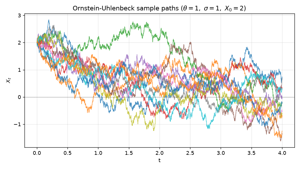

No individual path is predictable. But look at all $20{,}000$ of them at once and a pattern appears.

From One Path to a Density

Fix a time $t$ and forget the ordering of the paths. What we have is a cloud of values $X_t^{(1)}, X_t^{(2)}, \ldots$, one per path. Their histogram approximates a probability density $p(x, t)$: the probability of finding the process near $x$ at time $t$.

At $t = 0$ that density is a spike at $x = 2$, because every path starts there. As time runs, two things happen at once. The whole cloud drifts left toward zero, following the mean reversion. And it spreads out, because the noise accumulates. Eventually the inward pull and the outward spreading balance, and the density stops changing. That limiting shape is the stationary distribution.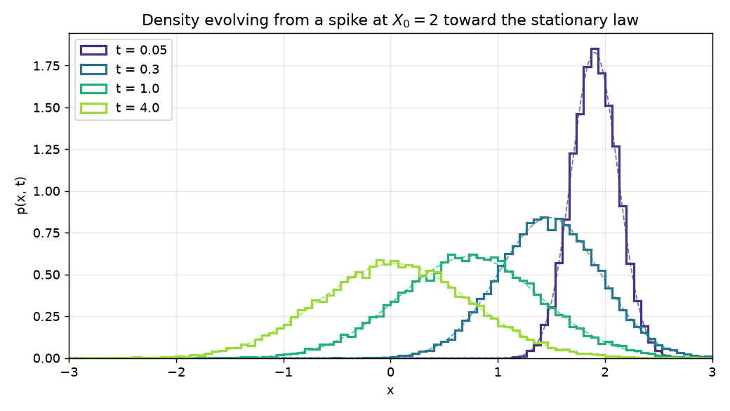

The question this note answers is: can we describe the movie of $p(x, t)$ directly, without simulating a single path? Yes. The density obeys a deterministic PDE, and that PDE is the Fokker-Planck equation.

Deriving the Fokker-Planck Equation from Ito's Lemma

The cleanest derivation uses a test function. Let $f$ be any smooth function that vanishes outside a bounded region. We track how the expectation $\mathbb{E}[f(X_t)]$ evolves, in two different ways, and match them.

Route one: apply Ito's lemma. For $dX_t = \mu, dt + \sigma, dW_t$, Ito's lemma says that the differential of $f(X_t)$ carries an extra second-order term that ordinary calculus would miss:

$$ df(X_t) = f'(X_t), dX_t + \tfrac{1}{2} f''(X_t), (dX_t)^2. $$

Using $(dX_t)^2 = \sigma^2, dt$ (the defining rule of Ito calculus, since $(dW_t)^2 = dt$),

$$ df(X_t) = \left[\mu, f'(X_t) + \tfrac{1}{2}\sigma^2 f''(X_t)\right] dt + \sigma f'(X_t), dW_t. $$

Take expectations. The $dW_t$ term has mean zero, so it drops out:

$$ \frac{d}{dt}, \mathbb{E}[f(X_t)] = \mathbb{E}!\left[\mu(X_t), f'(X_t) + \tfrac{1}{2}\sigma^2(X_t), f''(X_t)\right] = \int \left[\mu(x) f'(x) + \tfrac{1}{2}\sigma^2(x) f''(x)\right] p(x, t), dx. $$

Route two: differentiate under the integral. By definition $\mathbb{E}[f(X_t)] = \int f(x), p(x, t), dx$, so

$$ \frac{d}{dt}, \mathbb{E}[f(X_t)] = \int f(x), \frac{\partial p}{\partial t}, dx. $$

Match them. Set the two expressions equal and move all derivatives off $f$ using integration by parts. Because $f$ vanishes at the boundaries, every boundary term is zero:

$$ \int \mu f' p, dx = -\int f, \frac{\partial}{\partial x}(\mu p), dx, \qquad \int \tfrac{1}{2}\sigma^2 f'' p, dx = \int f, \frac{\partial^2}{\partial x^2}!\left(\tfrac{1}{2}\sigma^2 p\right) dx. $$

Substituting back, we get an identity that must hold for every test function $f$:

$$ \int f(x), \frac{\partial p}{\partial t}, dx = \int f(x)\left[-\frac{\partial}{\partial x}(\mu p) + \frac{\partial^2}{\partial x^2}!\left(\tfrac{1}{2}\sigma^2 p\right)\right] dx. $$

If two integrals agree against all test functions, their integrands agree. This gives the Fokker-Planck equation (also called the forward Kolmogorov equation):

$$ \boxed{;\frac{\partial p}{\partial t} = -\frac{\partial}{\partial x}\big[\mu(x, t), p\big] + \frac{\partial^2}{\partial x^2}!\left[\tfrac{1}{2}\sigma^2(x, t), p\right].;} $$

The derivation is worth pausing on. The first term came from the drift $\mu$ and is first order; the second came from the diffusion $\sigma$ and is second order, and it is there only because of the extra Ito term $\tfrac12 f''(dX)^2$. Without Ito calculus, the diffusion would vanish and the density would never spread. The whole "randomness" of the process lives in that one second-order term.

What the Equation Actually Says: Transport Plus Spreading

The Fokker-Planck equation is easier to read as a conservation law. Write it as

$$ \frac{\partial p}{\partial t} = -\frac{\partial J}{\partial x}, \qquad J(x, t) = \mu(x, t), p - \frac{\partial}{\partial x}!\left[\tfrac{1}{2}\sigma^2(x, t), p\right]. $$

Here $J$ is the probability current: the rate at which probability mass flows past the point $x$. The equation $\partial_t p = -\partial_x J$ is just the statement that probability is conserved. If more flows in than out at a point, the density there rises.

The current has two pieces, and they correspond exactly to the two forces in the SDE.

• Transport (drift). The term $\mu(x), p$ carries mass in the direction of the drift, like a wind blowing the density downstream. For the OU process $\mu = -\theta x$ blows everything toward the origin.
• Spreading (diffusion). The term $-\partial_x[\tfrac12\sigma^2 p]$ pushes mass from high-density regions to low-density ones, exactly like heat flowing from hot to cold. It is what turns a spike into a bell curve.

A stationary distribution $p_\infty$ is one where the movie stops: $\partial_t p = 0$, which means the current $J$ is constant. On the whole line, with density decaying to zero at infinity, that constant must be zero. Setting $J = 0$ for the OU process,

$$ -\theta x, p_\infty - \frac{\sigma^2}{2}, p_\infty' = 0 \quad\Longrightarrow\quad \frac{p_\infty'}{p_\infty} = -\frac{2\theta}{\sigma^2}, x \quad\Longrightarrow\quad p_\infty(x) \propto \exp!\left(-\frac{\theta x^2}{\sigma^2}\right). $$

That is a Gaussian with mean $0$ and variance $\sigma^2 / (2\theta)$. Drift and diffusion reach a truce, and the truce is a bell curve. With our numbers $\theta = \sigma = 1$, the stationary law is $\mathcal{N}(0, \tfrac12)$.

The Ornstein-Uhlenbeck Answer in Closed Form

The OU process is special: we can solve it exactly, which makes it the perfect test case. Because the drift is linear and the noise is additive, the transition density stays Gaussian for all time. Starting from a fixed $X_0 = x_0$, the process at time $t$ is normally distributed:

$$ X_t \sim \mathcal{N}\big(m(t),, v(t)\big), $$

$$ m(t) = x_0, e^{-\theta t}, \qquad v(t) = \frac{\sigma^2}{2\theta}\left(1 - e^{-2\theta t}\right). $$

The mean decays exponentially toward zero at rate $\theta$. The variance grows from $0$ up to the stationary value $\sigma^2 / (2\theta)$. Both limits match the picture: the cloud drifts to the origin and its width saturates.

You can verify these solve the Fokker-Planck equation by substitution, but it is more convincing to check them numerically, which is what the rest of the note does.

Hand Calculation with Real Numbers

Before writing any solver, pin down what the answer should be at a specific time, so we have something concrete to test against. Take $t = 1$ with $\theta = \sigma = 1$ and $x_0 = 2$.

Mean.

$$ m(1) = 2, e^{-1} = 2 \times 0.367879 = 0.735759. $$

Variance.

$$ v(1) = \frac{1}{2}\left(1 - e^{-2}\right) = \frac{1}{2}\left(1 - 0.135335\right) = \frac{1}{2}\times 0.864665 = 0.432332, $$

so the standard deviation is $\sqrt{0.432332} = 0.657520$.

Stationary check. As $t \to \infty$, $m(t) \to 0$ and $v(t) \to \tfrac12$, matching the $\mathcal{N}(0, \tfrac12)$ we derived from setting the current to zero. Its standard deviation is $\sqrt{0.5} = 0.707107$.

So at $t = 1$ the density should be a Gaussian centered at about $0.736$ with standard deviation about $0.658$, and by $t = 4$ it should be almost exactly $\mathcal{N}(0, \tfrac12)$. Keep these three numbers in mind; every method below has to reproduce them.

Solving the Fokker-Planck Equation from Scratch

We now solve the PDE numerically, without simulating any paths. Discretize $x$ on a grid and integrate the conservation law forward in time. The safe way to do this is to keep the flux form, so that the scheme conserves total probability by construction: compute the current $J$ on the cell faces (the midpoints between grid points), then update each cell by the difference of the fluxes on its two faces.

def solve_fokker_planck(mu, D, x, p0, T, dt):
    """Explicit finite-volume solver for  dp/dt = -d/dx(mu p) + d^2/dx^2(D p).
    mu(x): drift, D: constant diffusion sigma^2/2, x: grid, p0: initial density."""
    dx = x[1] - x[0]
    xf = 0.5 * (x[:-1] + x[1:])          # cell faces (midpoints)
    muf = mu(xf)
    p = p0.copy()
    n_steps = int(T / dt)
    for _ in range(n_steps):
        # probability current on the faces: transport minus diffusion
        J = muf * 0.5 * (p[:-1] + p[1:]) - D * (p[1:] - p[:-1]) / dx
        dpdt = np.zeros_like(p)
        dpdt[1:-1] = -(J[1:] - J[:-1]) / dx   # divergence of the current
        p = p + dt * dpdt
        p[0] = p[-1] = 0.0                     # absorbing far-field boundary
    return p

# grid and a narrow-Gaussian approximation to the initial spike at x0
x = np.linspace(-4, 4, 801)
dx = x[1] - x[0]
p0 = np.exp(-(x - x0) ** 2 / (2 * 0.01)) / np.sqrt(2 * np.pi * 0.01)

D = sigma_ou ** 2 / 2
dt_pde = 0.2 * dx ** 2 / D                 # diffusion stability limit (CFL)
p_pde = solve_fokker_planck(lambda z: -theta * z, D, x, p0, T=1.0, dt=dt_pde)

Two numerical points matter. First, the time step is bounded by a stability condition: for an explicit diffusion scheme, $\Delta t \lesssim \Delta x^2 / \sigma^2$. Push past it and the solution blows up into oscillations. Second, the initial spike at $x_0$ is approximated by a narrow Gaussian, because a true delta on a grid is a single spike that the scheme struggles with; the diffusion smooths this out almost immediately, so it does not affect the answer at $t = 1$.

Three Routes, One Answer

Now the payoff. We have three completely independent ways to get the density at $t = 1$:

1. Monte Carlo. Simulate many SDE paths with Euler-Maruyama and histogram their values at $t = 1$.
2. PDE. Solve the Fokker-Planck equation on a grid and read off $p(x, 1)$.
3. Closed form. Evaluate the exact Gaussian $\mathcal{N}(m(1), v(1))$.

from math import erf  # only for the analytic pdf below

# 1. Monte Carlo: reuse the trajectories, take the slice at t = 1
t_idx = int(1.0 / 1e-3)
mc_samples = traj[t_idx]

# 3. Closed-form transition density at t = 1
m1 = x0 * np.exp(-theta * 1.0)
v1 = (sigma_ou ** 2 / (2 * theta)) * (1 - np.exp(-2 * theta * 1.0))
analytic = np.exp(-(x - m1) ** 2 / (2 * v1)) / np.sqrt(2 * np.pi * v1)

print(f"analytic   mean={m1:.6f}  std={np.sqrt(v1):.6f}")
print(f"monte carlo mean={mc_samples.mean():.6f}  std={mc_samples.std():.6f}")
# PDE mean/std from the grid density p_pde
print(f"pde grid   mean={np.sum(x * p_pde) * dx:.6f}  "
      f"std={np.sqrt(np.sum((x - np.sum(x * p_pde) * dx) ** 2 * p_pde) * dx):.6f}")

All three report the same numbers we computed by hand, up to discretization error:

analytic    mean=0.735759  std=0.657520
monte carlo mean=0.738001  std=0.656903
pde grid    mean=0.735715  std=0.658482

Overlaid on the same axes, the Monte Carlo histogram, the PDE solution, and the analytic Gaussian sit on top of each other: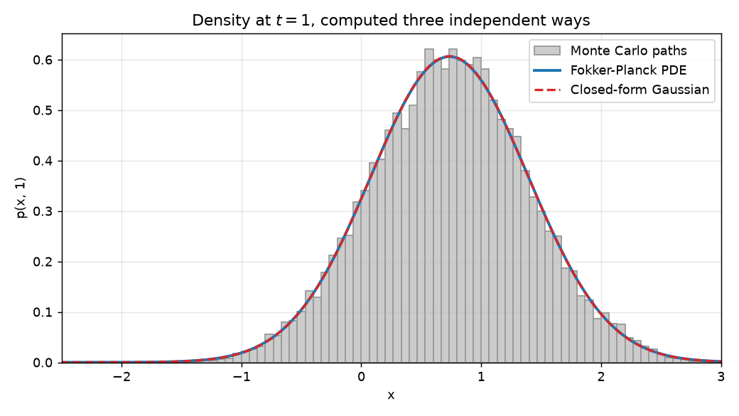

This is the moment where the theory becomes tangible. The Monte Carlo route never writes down a PDE; it just pushes paths forward and counts. The PDE route never simulates a path; it evolves a density on a grid. The closed form does neither; it solves the equation exactly. Three different arithmetic routes, one distribution, because the Fokker-Planck equation is precisely the deterministic law that the random ensemble obeys.

The Stationary Distribution

Let the same three methods run out to $t = 4$ and the density settles onto the stationary law $\mathcal{N}(0, \tfrac12)$ we derived by setting the probability current to zero: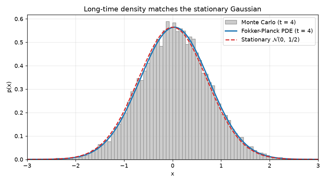

The process has forgotten its initial condition. Whether it started at $x_0 = 2$ or anywhere else, it relaxes to the same bell curve. That loss of memory, at rate $\theta$, is the defining property of a mean-reverting process, and the Fokker-Planck equation makes it quantitative.

Practical Points Worth Making Explicit

A few things trip people up when they take this beyond the OU example.

Stability of the explicit scheme. The time step must respect $\Delta t \lesssim \Delta x^2 / \sigma^2$. Halving the grid spacing quarters the allowed step. When this becomes expensive, implicit schemes (Crank-Nicolson) remove the restriction at the cost of solving a linear system each step.

Boundary conditions carry modelling meaning. We used an absorbing far-field boundary ($p = 0$), which is fine when the density decays anyway. But boundaries are not just numerics: a reflecting boundary (zero current, $J = 0$) models a wall the process cannot cross, while an absorbing boundary models a level at which the process is killed. In finance the absorbing case is exactly a barrier option or a default threshold.

State-dependent diffusion. When $\sigma$ depends on $x$, the second term is $\partial_x^2[\tfrac12 \sigma^2(x), p]$, and the $\sigma^2$ stays inside both derivatives. Geometric Brownian motion, $dX = \mu X, dt + \sigma X, dW$, is the standard example and underlies Black-Scholes. Getting that placement wrong is the most common error in writing down a Fokker-Planck equation.

Higher dimensions. In $d$ dimensions the drift becomes a vector and the diffusion a matrix $D = \tfrac12 \sigma \sigma^\top$, and the equation reads $\partial_t p = -\nabla!\cdot(\boldsymbol\mu p) + \nabla!\cdot(\nabla!\cdot(D, p))$. The grid solver stops scaling, and Monte Carlo becomes the practical method. That crossover is why simulation dominates high-dimensional problems.

The Big Picture

At this point the pieces should feel like one continuous argument rather than a definition dropped from the sky.

We started with an SDE, a rule for one random trajectory, and simulated it with Euler-Maruyama. One path is unpredictable, but the ensemble of paths forms a density $p(x, t)$. Applying Ito's lemma to a test function and integrating by parts turned the randomness of the SDE into a deterministic PDE for that density, the Fokker-Planck equation:

$$ \frac{\partial p}{\partial t} = -\frac{\partial}{\partial x}\big[\mu, p\big] + \frac{\partial^2}{\partial x^2}!\left[\tfrac{1}{2}\sigma^2, p\right]. $$

Reading it as a conservation law $\partial_t p = -\partial_x J$ exposed its two forces: drift transports probability, diffusion spreads it. Setting the current to zero gave the stationary distribution. And an Ornstein-Uhlenbeck example, solvable in closed form, let us check three independent routes, Monte Carlo, a from-scratch PDE solver, and the exact Gaussian, against the same hand-computed numbers.

So the SDE and the Fokker-Planck equation are two views of one process. The SDE is the microscopic rule for a single sample; the Fokker-Planck equation is the macroscopic law for the whole probability cloud. This is the same duality that runs through the rest of the stochastic toolkit: the forward Kolmogorov equation here evolves densities in time, while the backward Kolmogorov equation evolves expectations and is the object behind Feynman-Kac and option pricing.

I think this topic reads better when the SDE is taken as the starting point and the PDE is derived as its consequence, rather than the other way around. The mathematics carries the weight, the OU example makes the abstraction concrete, and the three-way agreement closes the loop.

If you think there is a better example, a cleaner derivation, or a natural extension, feel free to suggest it. From here the obvious next steps are the backward Kolmogorov equation and Feynman-Kac, Langevin dynamics as a sampler, and the jump from these scalar equations to their high-dimensional, matrix-diffusion form.