The butterfly diagram is usually the first thing people show you about the FFT. I think it should be the last. The FFT is nothing more than a fast way to compute the Discrete Fourier Transform, so none of it makes sense until the DFT does. And the DFT itself is easiest to see if you start from a sampled sound wave.
So this note goes:
$$ \text{sound wave} \to \text{samples} \to \text{DFT} \to \text{FFT} \to \text{spectrum}. $$
We build up the picture of sound as a sum of sinusoids, get the DFT as its discrete version, and then let the structure of the DFT matrix hand us the Cooley-Tukey FFT almost for free. At the end we run the whole thing on a real sound wave, implemented from scratch in Python.
Run it yourself. Every code block below is collected in a runnable Jupyter notebook: download
fft-sound-wave.ipynb. It only needsnumpyandmatplotlib(pip install numpy matplotlib), and runs top to bottom.
Start with a Sound Wave
Think of a pure musical tone. When a tuning fork vibrates at $440$ Hz, it displaces air molecules in a nearly sinusoidal way. The pressure at a fixed point in space looks like
$$ x(t) = A \cos(2\pi f t + \varphi), $$
with frequency $f = 440$ Hz, some amplitude $A$, and some phase $\varphi$.
A real sound is almost never a single sinusoid. A piano note at A4 contains the fundamental at $440$ Hz plus overtones at roughly $880$ Hz, $1320$ Hz, and so on, each with its own amplitude. More generally, any reasonable sound can be written as a sum of sinusoids:
$$ x(t) = \sum_{k} A_k \cos(2\pi f_k t + \varphi_k). $$
This is the Fourier picture. The time-domain view tells you what the waveform looks like at each instant. The frequency-domain view tells you which sinusoids, at which amplitudes and phases, combine to produce that waveform. The two views carry the same information but answer different questions.
On a computer, we never see $x(t)$ directly. We see samples. An analogue-to-digital converter records the pressure at a fixed sample rate $f_s$ (for example $44{,}100$ samples per second for CD audio), producing a finite sequence
$$ x_n = x(n / f_s), \qquad n = 0, 1, \ldots, N-1. $$
The question we really want to answer is: given these $N$ samples, which frequencies are present and how strong are they?
That question has a precise answer called the Discrete Fourier Transform.
From Fourier Series to the DFT
The continuous Fourier series says that a periodic signal can be written as a sum of complex exponentials:
$$ x(t) = \sum_{k=-\infty}^{\infty} c_k , e^{i 2\pi k t / T}, $$
where $T$ is the period. The coefficients $c_k$ tell us how much of each frequency $k/T$ is present. Complex exponentials show up here for a reason. Using Euler's formula,
$$ e^{i\theta} = \cos\theta + i\sin\theta, $$
a single complex exponential carries both a cosine and a sine at the same frequency. That packages amplitude and phase into one object and lets the math stay linear and clean.
Now discretize. Suppose we sample $x(t)$ at $N$ evenly spaced points over one period $T$, with spacing $\Delta t = T/N$. The samples are
$$ x_n = x(n \Delta t), \qquad n = 0, 1, \ldots, N-1. $$
The natural discrete analogue of the Fourier series uses $N$ complex exponentials,
$$ e^{i 2\pi k n / N}, \qquad k = 0, 1, \ldots, N-1, $$
as a basis for length-$N$ sequences. These discrete exponentials are orthogonal:
$$ \sum_{n=0}^{N-1} e^{i 2\pi k n / N} , e^{-i 2\pi \ell n / N} = \begin{cases} N & \text{if } k = \ell, \ 0 & \text{otherwise.} \end{cases} $$
Orthogonality is what makes the transform invertible. It also tells us the right formula for the coefficients, by projecting $x_n$ onto each basis vector.
This gives the Discrete Fourier Transform. For a sequence $x_0, x_1, \ldots, x_{N-1}$, define
$$ X_k = \sum_{n=0}^{N-1} x_n , e^{-i 2\pi k n / N}, \qquad k = 0, 1, \ldots, N-1. $$
And the inverse:
$$ x_n = \frac{1}{N} \sum_{k=0}^{N-1} X_k , e^{i 2\pi k n / N}. $$
Each $X_k$ is a complex number. Its magnitude $|X_k|$ tells us how strong the frequency component at bin $k$ is, and its phase $\arg X_k$ tells us where that sinusoid starts.
The frequency associated with bin $k$ is
$$ f_k = \frac{k}{N} f_s, $$
for $k = 0, 1, \ldots, N/2$, after which the bins fold by symmetry for real inputs. The highest frequency we can resolve is $f_s / 2$, the Nyquist frequency. Anything above that aliases down into lower bins, which is why sample rate matters.
What the Transform Actually Does: The Winding View
The formula for $X_k$ is easy to write down but easy to stare at without seeing anything. Before we optimize how to compute it, here is a different perspective on what it computes, one that makes the whole transform intuitive.
Look again at a single term. The factor
$$ e^{-i 2\pi k n / N} $$
is a unit vector in the complex plane that rotates clockwise as $n$ advances. Multiplying the signal $x_n$ by it winds the signal around the origin at a winding rate set by $k$: small $k$ winds slowly, large $k$ winds fast. The sum over $n$ then just adds up all those wound points, and dividing by $N$ gives their center of mass (their average position).
So $X_k / N$ is literally: take the signal, wrap it around a circle at rate $k$, and find the center of mass of the resulting curve.
Now the key effect. When the winding rate matches a frequency that is actually present in the signal, the signal's peaks land on the same side of the circle on every turn. The wound points pile up on one side, and their center of mass sits far from the origin: a large $|X_k|$. When the winding rate does not match, the peaks land at different angles each turn, spread evenly around the circle, and cancel. The center of mass collapses to near zero.
To see it, here is a simple two-component signal (a $2$ Hz plus a $3$ Hz cosine, chosen at low frequencies purely so the winding is visible) wound at four different rates: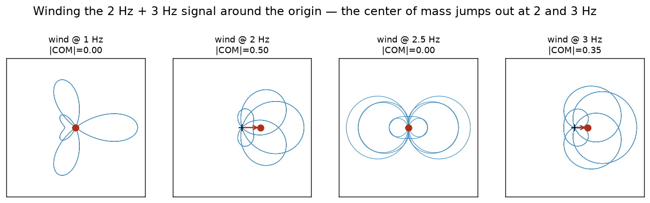
Sweep the winding rate continuously and record how far the center of mass sits from the origin at each rate, and you trace out the Fourier transform magnitude directly: flat and near zero everywhere except sharp bumps at exactly the frequencies the signal contains.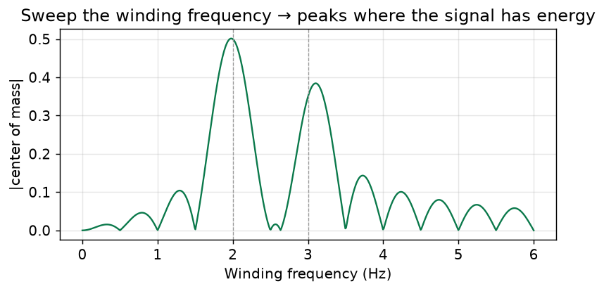
The same picture is clearer in three dimensions. Stack each wound copy of the signal along a third axis given by its winding frequency. Most slices are balanced loops centered on the axis; only at the true frequencies does the center of mass bulge outward.
That is the one-sentence summary of the entire transform: the DFT measures how well the signal lines up with a corkscrew of each frequency. The complex exponential $e^{-i 2\pi k n / N}$ is that corkscrew, and the sum is the alignment score. Everything that follows (the matrix form, the even/odd split, the butterflies) is just machinery for computing all $N$ of these alignment scores quickly.
The DFT as a Matrix
Define the primitive root of unity
$$ \omega_N = e^{-i 2\pi / N}. $$
Then
$$ X_k = \sum_{n=0}^{N-1} x_n , \omega_N^{kn}. $$
Let $F_N$ be the $N \times N$ matrix with entries $(F_N)_{k,n} = \omega_N^{kn}$. Then the DFT is just a matrix-vector product:
$$ X = F_N x. $$
A matrix-vector product with a dense $N \times N$ matrix takes $O(N^2)$ multiplications and additions. For a one-second CD-quality audio frame with $N = 44{,}100$ samples that is about $2 \times 10^9$ operations per frame. Doable, but clearly wasteful if the matrix has structure.
It does. The matrix $F_N$ is extremely structured, because $\omega_N$ is a root of unity. The FFT is the algorithm that exploits that structure.
The FFT Idea: Split Into Even and Odd
The Cooley-Tukey FFT is a divide-and-conquer algorithm. Assume $N$ is a power of two (we can always zero-pad to get there). Split the input sequence by index parity:
$$ \text{even part: } ; x_0, x_2, x_4, \ldots, x_{N-2}, $$
$$ \text{odd part: } ; x_1, x_3, x_5, \ldots, x_{N-1}. $$
Now rewrite $X_k$ by separating even and odd indices:
$$ X_k ;=; \sum_{m=0}^{N/2 - 1} x_{2m} , e^{-i 2\pi k (2m) / N} ;+; \sum_{m=0}^{N/2 - 1} x_{2m+1} , e^{-i 2\pi k (2m+1) / N}. $$
Pull out the extra factor in the odd sum:
$$ X_k ;=; \sum_{m=0}^{N/2 - 1} x_{2m} , e^{-i 2\pi k m / (N/2)} ;+; e^{-i 2\pi k / N} \sum_{m=0}^{N/2 - 1} x_{2m+1} , e^{-i 2\pi k m / (N/2)}. $$
Now look carefully at each sum. Each one is itself a DFT, of length $N/2$. Let
$$ E_k = \sum_{m=0}^{N/2 - 1} x_{2m} , e^{-i 2\pi k m / (N/2)}, \qquad O_k = \sum_{m=0}^{N/2 - 1} x_{2m+1} , e^{-i 2\pi k m / (N/2)}. $$
Then
$$ X_k = E_k + e^{-i 2\pi k / N} , O_k. $$
The quantity $e^{-i 2\pi k / N}$ is usually written
$$ W_N^k = e^{-i 2\pi k / N} $$
and called a twiddle factor. It is the bookkeeping that corrects for the shift between even and odd indices.
The Butterfly: Two Outputs for the Price of One
We have computed $X_k$ in terms of $E_k$ and $O_k$ for $k = 0, 1, \ldots, N/2 - 1$. What about $k = N/2, N/2+1, \ldots, N-1$?
Use the periodicity of $E_k$ and $O_k$. Both are length-$N/2$ DFTs, so
$$ E_{k + N/2} = E_k, \qquad O_{k + N/2} = O_k. $$
The twiddle factor shifts by a sign:
$$ W_N^{k + N/2} = e^{-i 2\pi (k + N/2) / N} = e^{-i 2\pi k / N} e^{-i\pi} = -W_N^k. $$
Combining these,
$$ X_k = E_k + W_N^k , O_k, $$
$$ X_{k + N/2} = E_k - W_N^k , O_k. $$
That pair of equations is one butterfly. From two inputs $E_k$ and $O_k$ (and a precomputed twiddle), we produce two outputs $X_k$ and $X_{k+N/2}$ using one complex multiplication and two complex additions. We reuse work instead of redoing it.
At this point the whole algorithm is already visible. Compute two $N/2$-point DFTs. Combine them with $N/2$ butterflies to produce the $N$-point DFT. Recurse on each half.
Complexity: Why It Is $O(N \log N)$
Let $T(N)$ be the number of operations to compute an $N$-point DFT using this recursion. We do:
- Two DFTs of size $N/2$, each costing $T(N/2)$.
- $N/2$ butterflies to combine them, each a constant amount of work. So $O(N)$ total for the combine step.
That gives the recurrence
$$ T(N) = 2 T(N/2) + cN, $$
with $T(1) = O(1)$, for some constant $c$.
Unroll the recurrence:
$$ T(N) ;=; 2T(N/2) + cN ;=; 4 T(N/4) + 2cN ;=; 8 T(N/8) + 3cN ;=; \ldots $$
After $\log_2 N$ levels of unrolling we reach $T(1)$, and each level contributes $cN$ work:
$$ T(N) = N \cdot T(1) + cN \log_2 N = O(N \log N). $$
Compare that to the naive DFT. For $N = 2^{20} \approx 10^6$:
$$ N^2 = 10^{12}, \qquad N \log_2 N \approx 2 \times 10^7. $$
Five orders of magnitude. That is the whole reason real-time audio processing, modern communications, and large-scale scientific computing are tractable.
A Worked Example: N = 4
To see the recursion concretely, take $N = 4$ with input $x = (x_0, x_1, x_2, x_3)$.
The even part is $(x_0, x_2)$, and the odd part is $(x_1, x_3)$. Both are length-2 DFTs.
For a length-2 DFT with input $(a, b)$:
$$ Y_0 = a + b, \qquad Y_1 = a - b, $$
which is itself one butterfly with twiddle $W_2^0 = 1$.
So the two half-DFTs give
$$ E_0 = x_0 + x_2, \quad E_1 = x_0 - x_2, $$
$$ O_0 = x_1 + x_3, \quad O_1 = x_1 - x_3. $$
The twiddle factors at size $N=4$ are $W_4^0 = 1$ and $W_4^1 = e^{-i\pi/2} = -i$. Combining:
$$ X_0 = E_0 + W_4^0 , O_0 = (x_0 + x_2) + (x_1 + x_3), $$
$$ X_1 = E_1 + W_4^1 , O_1 = (x_0 - x_2) - i(x_1 - x_3), $$
$$ X_2 = E_0 - W_4^0 , O_0 = (x_0 + x_2) - (x_1 + x_3), $$
$$ X_3 = E_1 - W_4^1 , O_1 = (x_0 - x_2) + i(x_1 - x_3). $$
Four outputs, built from two pairs of butterflies. You can check by hand that these match $X_k = \sum_n x_n \omega_4^{kn}$ directly. This is the full FFT, in miniature.
Hand Calculation with Real Numbers
The symbolic form is useful, but it is more convincing to watch the recursion run on actual numbers. Take the concrete input
$$ x = (x_0, x_1, x_2, x_3) = (1, 2, 3, 4). $$
Following the principle from the previous section step by step.
Step 1. Split by parity.
$$ \text{even: } (x_0, x_2) = (1, 3), \qquad \text{odd: } (x_1, x_3) = (2, 4). $$
Step 2. Length-2 DFT of each half. Using $Y_0 = a + b$, $Y_1 = a - b$:
$$ E_0 = 1 + 3 = 4, \qquad E_1 = 1 - 3 = -2, $$
$$ O_0 = 2 + 4 = 6, \qquad O_1 = 2 - 4 = -2. $$
Step 3. Twiddle factors at $N = 4$.
$$ W_4^0 = e^{0} = 1, \qquad W_4^1 = e^{-i\pi/2} = -i. $$
Step 4. Apply the butterfly equations. Using $X_k = E_k + W_4^k O_k$ and $X_{k+2} = E_k - W_4^k O_k$:
$$ X_0 = E_0 + W_4^0 , O_0 = 4 + (1)(6) = 10, $$
$$ X_1 = E_1 + W_4^1 , O_1 = -2 + (-i)(-2) = -2 + 2i, $$
$$ X_2 = E_0 - W_4^0 , O_0 = 4 - 6 = -2, $$
$$ X_3 = E_1 - W_4^1 , O_1 = -2 - (-i)(-2) = -2 - 2i. $$
So by hand,
$$ X = (10,; -2 + 2i,; -2,; -2 - 2i). $$
Step 5. Cross-check with code. Running the same input through numpy and our from-scratch implementations should produce exactly the same vector:
import numpy as np

x = np.array([1, 2, 3, 4], dtype=complex)

print("numpy  :", np.fft.fft(x))
print("naive  :", naive_dft(x))
print("fft_rec:", fft_recursive(x))
Expected output (up to floating-point error):
numpy  : [10.+0.j -2.+2.j -2.+0.j -2.-2.j]
naive  : [10.+0.j -2.+2.j -2.+0.j -2.-2.j]
fft_rec: [10.+0.j -2.+2.j -2.+0.j -2.-2.j]
Three different routes, one answer. The naive DFT sums all $N^2 = 16$ terms directly. The recursive FFT computes two length-2 DFTs and combines them with two butterflies, using far fewer operations. Both recover the same spectrum because they are computing the same mathematical object, just through different arithmetic paths.
This is the moment where the principle becomes tangible. Even/odd split, two half-DFTs, twiddle factor, butterfly. Four equations, one vector of outputs. Scale the same pattern recursively to $N = 8, 16, \ldots, 2^{20}$ and you have the full FFT.
From Scratch in Python: Naive DFT and Recursive FFT
The fastest way to internalize this is to implement both and watch them agree.
Start with the naive DFT, a direct translation of the definition:
import numpy as np

def naive_dft(x):
    x = np.asarray(x, dtype=complex)
    N = x.shape[0]
    n = np.arange(N)
    k = n.reshape((N, 1))
    M = np.exp(-2j * np.pi * k * n / N)
    return M @ x
Now the recursive Cooley-Tukey FFT. It assumes $N$ is a power of two. When $N$ drops to a small base case we hand off to the naive DFT, which is fine for tiny sizes:
def fft_recursive(x):
    x = np.asarray(x, dtype=complex)
    N = x.shape[0]

    if N & (N - 1):
        raise ValueError("Length of input must be a power of 2.")

    if N <= 2:
        return naive_dft(x)

    X_even = fft_recursive(x[0::2])
    X_odd = fft_recursive(x[1::2])

    k = np.arange(N // 2)
    twiddle = np.exp(-2j * np.pi * k / N)

    return np.concatenate([X_even + twiddle * X_odd,
                           X_even - twiddle * X_odd])
Check agreement with numpy.fft.fft on random input:
rng = np.random.default_rng(0)
x = rng.standard_normal(1024)

X_naive = naive_dft(x)
X_fft = fft_recursive(x)
X_np = np.fft.fft(x)

print(np.allclose(X_naive, X_np))
print(np.allclose(X_fft, X_np))
Both should print True up to floating-point error. The three implementations compute the same mathematical object. The FFT just computes it faster.
A Real Sound-Wave Example
Now the payoff. We construct a synthetic sound wave made of three tones, sample it, and recover those tones from the samples using the FFT.
import numpy as np
import matplotlib.pyplot as plt

sample_rate = 8000
duration = 1.0
N = int(sample_rate * duration)
t = np.arange(N) / sample_rate

x = (1.0 * np.sin(2 * np.pi * 220 * t)
     + 0.6 * np.sin(2 * np.pi * 440 * t)
     + 0.3 * np.sin(2 * np.pi * 880 * t))

x += 0.05 * np.random.default_rng(0).standard_normal(N)
The signal x contains a strong $220$ Hz tone, a medium $440$ Hz tone, a weaker $880$ Hz tone, and a small amount of noise.
In the time domain the waveform looks periodic but visually messy. That is expected. Time domain is not the right view for this question.
Now apply the FFT. Because N = 8000 is not a power of two, we either zero-pad up to the next power of two or use a mixed-radix FFT. For this note we will zero-pad, which is also a common practical trick to improve bin resolution:
def next_pow2(n):
    return 1 << (n - 1).bit_length()

N_pad = next_pow2(N)
x_pad = np.zeros(N_pad)
x_pad[:N] = x

X = fft_recursive(x_pad)
magnitude = np.abs(X) / N
freqs = np.arange(N_pad) * sample_rate / N_pad

half = N_pad // 2
plt.plot(freqs[:half], magnitude[:half])
plt.xlabel("Frequency (Hz)")
plt.ylabel("Magnitude")
plt.title("Magnitude spectrum of the synthetic sound wave")
plt.grid(True)
plt.show()
The spectrum shows three clean peaks, at $220$, $440$, and $880$ Hz, with heights roughly proportional to the amplitudes we put in. The noise spreads thinly across all other bins and stays small.
That is the central picture. The time-domain view showed an oscillating mess. The frequency-domain view recovers exactly the three tones we synthesized, because that is what the DFT does. The FFT just made the computation fast enough to be practical on a full second of audio.
Naive DFT vs FFT: Timing
To make the complexity story concrete, it helps to time both implementations on increasing input sizes. The naive DFT should grow quadratically, and the recursive FFT should grow close to linearly in $N \log N$:
import time

sizes = [2**k for k in range(6, 13)]
naive_times = []
fft_times = []

for N in sizes:
    x = np.random.default_rng(0).standard_normal(N)

    t0 = time.perf_counter()
    naive_dft(x)
    naive_times.append(time.perf_counter() - t0)

    t0 = time.perf_counter()
    fft_recursive(x)
    fft_times.append(time.perf_counter() - t0)

plt.loglog(sizes, naive_times, marker="o", label="naive DFT")
plt.loglog(sizes, fft_times, marker="o", label="recursive FFT")
plt.xlabel("N")
plt.ylabel("Time (s)")
plt.title("Runtime: naive DFT vs recursive FFT")
plt.legend()
plt.grid(True, which="both")
plt.show()
On a log-log plot, the naive DFT has slope close to $2$ and the recursive FFT has slope close to $1$. That is the $O(N^2)$ versus $O(N \log N)$ gap, visualized directly.
Sampling, Nyquist, and Aliasing
A few practical points are worth making explicit, because they trip people up in real audio code.
The highest frequency the DFT can represent is the Nyquist frequency $f_s / 2$. At sample rate $8000$ Hz, that is $4000$ Hz. Any signal component above that frequency does not simply vanish. It aliases down into a lower bin and corrupts the spectrum. That is why audio is low-pass filtered before sampling.
For real-valued inputs, the spectrum is conjugate-symmetric: $X_{N-k} = \overline{X_k}$. So the second half of the DFT output carries no new information. In practice we only plot bins $0$ through $N/2$.
The frequency resolution of the DFT is $f_s / N$. Longer windows give finer frequency resolution but worse time resolution. This trade-off is exactly why short-time Fourier transforms and wavelets exist.
Windowing and Spectral Leakage
If the signal frequency does not land exactly on a DFT bin, its energy spreads into neighboring bins. This is called spectral leakage, and it is a property of the DFT, not a bug. Leakage is reduced by multiplying the signal by a smooth window function before the transform:
window = np.hanning(N)
x_windowed = x * window
A Hann window tapers the signal smoothly to zero at both ends, which suppresses the discontinuity that causes leakage. The trade-off is a slight widening of each spectral peak. For most audio applications this is a good deal.
Real Input: A Slightly Faster Variant
When the input is real, numpy.fft.rfft returns only the non-redundant half of the spectrum and is about twice as fast as the full complex FFT. In from-scratch code the same idea can be implemented by exploiting the conjugate symmetry directly. For production use, numpy.fft.rfft or any mature FFT library (FFTW, PocketFFT, cuFFT) is almost always the right choice. The recursive implementation above is for understanding, not for speed.
The Big Picture
At this point the whole thing should feel like one continuous argument, not three unrelated algorithms.
We started with a sound wave in the time domain and asked which frequencies it contains. Sampling gave us a finite sequence $x_n$. Projecting that sequence onto a basis of complex exponentials gave the DFT:
$$ X_k = \sum_{n=0}^{N-1} x_n , e^{-i 2\pi k n / N}. $$
The DFT is a linear map, so it can be written as a matrix product $X = F_N x$. Computed naively, that is $O(N^2)$.
We then exploited the structure of $F_N$. The roots of unity satisfy a recursion, so the $N$-point DFT splits into two $N/2$-point DFTs combined by $N/2$ butterflies. That gives the recurrence $T(N) = 2T(N/2) + O(N)$ and the complexity $O(N \log N)$.
Finally, we tested the whole pipeline on a synthetic sound wave and recovered the three input tones as three clean peaks in the magnitude spectrum.
So in the end, the DFT is the definition and the FFT is the algorithm. The DFT says what we want. The FFT says how to get it quickly. The exponential keeps showing up for the same reason it does in logistic and softmax regression: it is the right basis when the underlying object has multiplicative structure. Roots of unity are multiplicative. Splitting them in half, again and again, is exactly what turns $N^2$ into $N \log N$.
If I keep going with this, the next stops are the short-time Fourier transform and spectrograms, and after that the jump from Fourier bases to wavelets. Corrections and better examples are welcome in the comments.